Trie Data Structures: Prefix Trees, Implementation & Use Cases
By
Liz Fujiwara
•
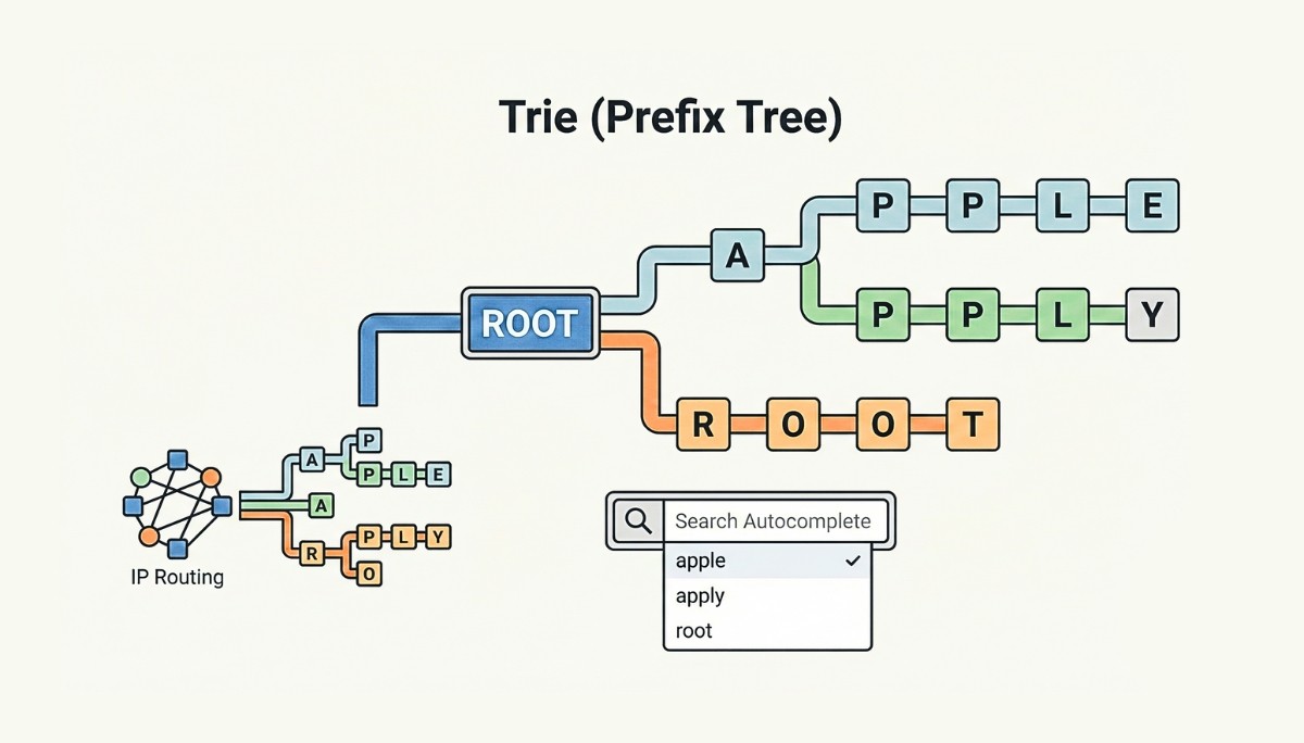
Every time you type “app” into a search box and instantly see suggestions like “apple,” “application,” and “approach,” you’re witnessing the power of trie data structures in action. This lightning-fast autocomplete functionality isn’t magic; it’s the result of a carefully designed tree data structure optimized specifically for string processing and prefix-based searches.
A trie, also known as a prefix tree or digital tree, is one of the fundamental data structures that every developer should understand. Unlike traditional hash tables or binary search trees, tries excel at storing and retrieving strings efficiently by leveraging the natural hierarchical relationship between words that share common prefixes.
Ensure strong integration by establishing clear communication protocols, structured onboarding, defined collaboration practices, and overlapping work hours for real-time coordination.
Key Takeaways
Tries store strings efficiently by sharing common prefixes, enabling fast O(m) insert, search, and delete operations and making them ideal for autocomplete and spell-checking systems.
They outperform hash tables for prefix-based queries, maintain lexicographical order, and offer sorted traversal without additional sorting overhead.
Advanced variants like radix trees and Patricia trees improve memory efficiency for large or sparse datasets, supporting real-world applications from search engines to IP routing.
What is a Trie Data Structure?
A trie data structure is a specialized tree-based data structure designed specifically for storing and retrieving strings efficiently. The name “trie” derives from the word “retrieval,” highlighting its primary purpose of enabling rapid string retrieval operations. This fundamental data structure is also commonly referred to as a prefix tree or digital tree, names that better describe its hierarchical organization of string data.
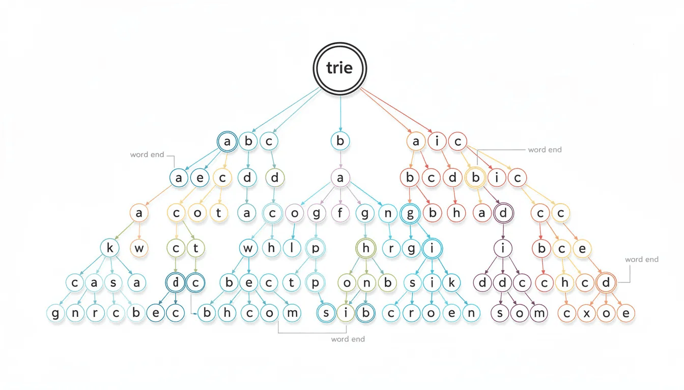
At its core, a trie organizes strings by breaking them down into their individual characters, with each character represented by a node in the tree structure. The key insight behind tries is that strings sharing common prefixes can share the same path from the root node, dramatically reducing memory usage and enabling efficient prefix-based operations.
The architecture of a trie consists of nodes connected by edges, with one critical feature: a single root node that represents an empty string and serves as the starting point for all operations. From this root node, each edge represents a character, and each path from the root to any other node represents a complete string prefix. When a complete word ends at a particular node, that node is marked with a special flag indicating a valid word termination.
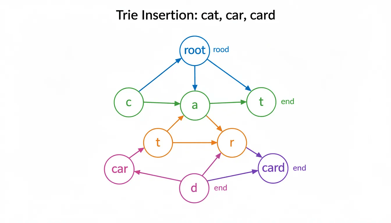
Consider how the words “cat,” “car,” and “card” would be stored in a trie structure. Starting from the root node, all three words share the path for ‘c’ and ‘a’. The trie then branches at the third character: one path follows ‘r’ for “car” and “card,” while another follows ‘t’ for “cat.” This shared prefix storage is what makes tries so memory-efficient for datasets with many related words.
Each node in a trie structure typically contains two main components: a collection of child pointers (usually an array or hash map) and a boolean flag indicating whether any string ends at that particular node. For English text processing, nodes commonly use an array of 26 pointers corresponding to lowercase letters a–z, where the index represents the character (‘a’ at index 0, ‘b’ at index 1, and so on).
The beauty of this organization becomes apparent when you need to find all words starting with a given prefix. Instead of checking every stored word individually, you simply traverse the trie following the prefix characters, then explore all possible paths from that endpoint to collect matching words.
How Trie Operations Work
Understanding how tries manipulate string data requires examining their four fundamental operations: insertion, search, deletion, and prefix search. Each operation leverages the tree structure’s character-by-character navigation to achieve optimal performance.
Insertion Operation
The insertion operation builds a trie by adding new words one character at a time, creating new nodes as needed while reusing existing paths for shared prefixes. This process starts at the root node and follows a systematic approach for each character in the string being inserted.
When inserting a string word into a trie, the algorithm begins by setting a pointer to the root node. For each character in the string, it calculates the corresponding index (typically using char - 'a' for lowercase letters) and checks whether a child node exists at that position. If no child node exists, the algorithm creates a new node and establishes the connection. If a child node already exists, the algorithm simply moves to that existing node.
Let’s trace through inserting “cat,” “car,” and “card” into an initially empty trie to illustrate this process:
Inserting “cat”: Starting from the root, create a new node for ‘c’ at index 2, then a new node for ‘a’ at index 0, then a new node for ‘t’ at index 19. Mark the final node as the end of a word.
Inserting “car”: From root, follow the existing path through ‘c’ and ‘a’ (reusing the shared prefix), then create a new node for ‘r’ at index 17. Mark this node as word termination.
Inserting “card”: Follow the existing path through ‘c’, ‘a’, and ‘r’, then create a new node for ‘d’ at index 3 and mark it as a word ending.
def insert(self, word):
current = self.root
for char in word:
index = ord(char) - ord('a')
if not current.children[index]:
current.children[index] = TrieNode()
current = current.children[index]
current.is_end_of_word = True
The time complexity for insertion is O(m) where m represents the length of the string being inserted, as the algorithm must process each character exactly once. The space complexity depends on how many new nodes must be created, which varies based on existing shared prefixes.
Search Operation
Searching for a string in a trie involves traversing the tree following the path defined by each character in the target string. This operation distinguishes between finding a valid word versus finding just a prefix that exists in the trie structure.
The search algorithm maintains a current node pointer that starts at the root. For each character in the search string, it calculates the character’s index and attempts to follow the corresponding child pointer. If any character leads to a null link (no child node exists), the search returns false immediately since the string doesn’t exist in the trie.
When the algorithm successfully processes all characters in the search string, it must check whether the final node has its end-of-word flag set to true. This distinction is crucial because a string might exist as a prefix in the trie without being a complete word stored in the structure.
def search(self, word):
current = self.root
for char in word:
index = ord(char) - ord('a')
if not current.children[index]:
return False
current = current.children[index]
return current.is_end_of_word
For example, searching for “car” in our trie would traverse through ‘c’, ‘a’, and ‘r’, reaching a node marked as a word ending, so the search returns true. However, searching for “ca” would traverse through ‘c’ and ‘a’ but reach a node not marked as a word ending, so the search would return false even though “ca” exists as a prefix.
Deletion Operation
Deletion in tries requires careful handling to avoid breaking other words that share prefixes with the string being deleted. The operation must remove nodes only when they’re no longer needed by any other word in the trie structure.
Three scenarios arise when deleting a string from a trie:
Unique key: The string doesn’t serve as a prefix for any other word, allowing safe removal of all its unique nodes.
Key as prefix: The string being deleted is a prefix of another longer word, requiring only the removal of its end-of-word marker.
Key with prefix: The string shares a prefix with other words, requiring careful removal of only the unique suffix portion.
The deletion algorithm typically uses a recursive approach that processes characters from the end of the string backward, cleaning up nodes that are no longer necessary while preserving shared prefixes.
def delete(self, word):
def _delete_helper(node, word, index):
if index == len(word):
if not node.is_end_of_word:
return False # Word doesn't exist
node.is_end_of_word = False
return not any(node.children) and not node.is_end_of_word
char_index = ord(word[index]) - ord('a')
child_node = node.children[char_index]
if not child_node:
return False # Word doesn't exist
should_delete_child = _delete_helper(child_node, word, index + 1)
if should_delete_child:
node.children[char_index] = None
return not any(node.children) and not node.is_end_of_word
return False
_delete_helper(self.root, word, 0)
Prefix Search Operation
One of the most powerful features of tries is their ability to efficiently find all words that start with a given prefix. This operation combines the traversal logic of search with a collection phase that gathers all valid word endings from the prefix endpoint.
The prefix search algorithm first navigates to the node representing the end of the given prefix using the same traversal logic as a regular search. If the prefix doesn’t exist in the trie (indicated by encountering a null link), the operation returns an empty result.
Once the prefix endpoint is located, the algorithm performs a depth-first traversal of all subtrees rooted at that node, collecting complete words by concatenating the prefix with each valid path to a word ending.
def words_with_prefix(self, prefix):
current = self.root
# Navigate to prefix endpoint
for char in prefix:
index = ord(char) - ord('a')
if not current.children[index]:
return [] # Prefix doesn't exist
current = current.children[index]
# Collect all words from this point
results = []
if current.is_end_of_word:
results.append(prefix)
def dfs(node, current_word):
for i, child in enumerate(node.children):
if child:
char = chr(ord('a') + i)
new_word = current_word + char
if child.is_end_of_word:
results.append(new_word)
dfs(child, new_word)
dfs(current, prefix)
return results
This prefix search capability is what makes tries exceptionally powerful for autocomplete systems, where users expect instant suggestions based on partial input.
Time and Space Complexity Analysis
Understanding the performance characteristics of trie operations is crucial for determining when tries offer advantages over alternative data structures. The complexity analysis reveals both the strengths and limitations of this approach to string storage.
Time Complexity Analysis
All primary trie operations, insertion, search, and deletion, exhibit O(m) time complexity, where m represents the length of the string being processed. This linear relationship with string length is independent of the total number of words stored in the trie, providing consistent performance regardless of trie size.
For prefix search operations, the time complexity is O(p + n), where p is the length of the prefix and n is the number of words that share that prefix. The initial traversal to reach the prefix endpoint requires O(p) time, while collecting all matching words requires time proportional to the number of results.
This performance characteristic contrasts favorably with hash tables, which provide O(1) average-case lookup for complete keys but require O(n) time for prefix searches, where n represents the total number of stored strings. Binary search trees offer O(log n) lookup time but still require O(n) time for prefix collection without additional indexing.
Space Complexity Analysis
The space complexity of tries depends heavily on the characteristics of the stored data, particularly the degree of prefix sharing among stored strings. In the worst case, where no strings share common prefixes, a trie requires O(ALPHABET_SIZE × N × M) space, where N is the number of strings and M is the average string length.
However, real-world datasets often exhibit significant prefix sharing, especially in applications like dictionaries or autocomplete systems. In such cases, the space complexity becomes much more favorable, approaching O(total_characters_across_all_unique_prefixes).
Consider the memory usage for a single trie node: each node typically requires space for an array or hash map of child pointers plus a boolean flag. For a 26-character English alphabet implementation, each node needs approximately 26 pointers plus metadata, which can total 104-112 bytes in languages like Java due to object overhead.
Comparison with Alternative Structures
Data Structure | Search Time | Prefix Search | Space Efficiency | Ordered Traversal |
Trie | O(m) | O(p + k) | High for shared prefixes | Yes |
Hash Table | O(1) avg | O(n) | Moderate | No |
Binary Search Tree | O(log n) | O(log n + k) | High | Yes |
Array | O(n) | O(n) | Highest | Only if sorted |
The table reveals that tries excel in scenarios requiring frequent prefix operations while maintaining reasonable space efficiency for datasets with common prefixes. The consistent O(m) performance makes tries particularly attractive for applications with predictable string lengths.
Best and Worst Case Scenarios
Tries perform optimally when processing datasets with many shared prefixes, such as:
Dictionary words in natural languages
File path hierarchies
DNA sequences with repeated patterns
Phone number databases with area code groupings
Conversely, tries may be less efficient for:
Random strings without common prefixes
Very short strings where overhead dominates
Memory-constrained environments with sparse datasets
Applications requiring only exact match lookups
Implementation Guide
Implementing a trie data structure requires careful attention to both the node architecture and the class interface. This section provides complete implementation examples that demonstrate best practices for building production-ready trie systems.
Basic Trie Node Structure
The foundation of any trie implementation is the node structure that represents individual characters and maintains the tree relationships. A well-designed trie node balances memory efficiency with operational performance.
class TrieNode:
def __init__(self):
self.children = [None] * 26 # For lowercase a-z
self.is_end_of_word = False
class TrieNode:
def __init__(self):
self.children = {} # More memory efficient for sparse data
self.is_end_of_word = False
The array-based approach provides constant-time character access using index arithmetic (ord(char) - ord('a')), while the dictionary approach conserves memory space when dealing with sparse character sets or Unicode text. The choice between these approaches depends on your specific use case and memory constraints.
For applications requiring additional metadata, nodes can be extended to store associated values:
class TrieNode:
def __init__(self):
self.children = [None] * 26
self.is_end_of_word = False
self.word_count = 0 # Track frequency
self.associated_value = None # Store additional data
Complete Trie Class Implementation
A complete trie implementation encapsulates all necessary operations while providing a clean interface for client code. Here’s a comprehensive implementation that demonstrates proper error handling and optimization techniques:
class Trie:
def __init__(self):
self.root = TrieNode()
self.size = 0
def insert(self, word):
"""Insert a word into the trie."""
if not word:
return False
current = self.root
for char in word.lower():
if not char.isalpha():
return False # Only accept alphabetic characters
index = ord(char) - ord('a')
if not current.children[index]:
current.children[index] = TrieNode()
current = current.children[index]
if not current.is_end_of_word:
current.is_end_of_word = True
self.size += 1
return True
return False # Word already exists
def search(self, word):
"""Search for a complete word in the trie."""
node = self._find_node(word)
return node is not None and node.is_end_of_word
def starts_with(self, prefix):
"""Check if any word starts with the given prefix."""
return self._find_node(prefix) is not None
def _find_node(self, word):
"""Helper method to find the node corresponding to a word/prefix."""
current = self.root
for char in word.lower():
index = ord(char) - ord('a')
if not current.children[index]:
return None
current = current.children[index]
return current
def get_words_with_prefix(self, prefix):
"""Return all words that start with the given prefix."""
prefix_node = self._find_node(prefix)
if not prefix_node:
return []
results = []
if prefix_node.is_end_of_word:
results.append(prefix)
self._collect_words(prefix_node, prefix, results)
return sorted(results)
def _collect_words(self, node, current_word, results):
"""Recursively collect all words from a given node."""
for i in range(26):
if node.children[i]:
char = chr(ord('a') + i)
new_word = current_word + char
if node.children[i].is_end_of_word:
results.append(new_word)
self._collect_words(node.children[i], new_word, results)
def delete(self, word):
"""Delete a word from the trie."""
if not self.search(word):
return False
def _delete_recursive(node, word, index):
if index == len(word):
node.is_end_of_word = False
return not any(node.children)
char_index = ord(word[index]) - ord('a')
child_node = node.children[char_index]
should_delete_child = _delete_recursive(child_node, word, index + 1)
if should_delete_child:
node.children[char_index] = None
return not node.is_end_of_word and not any(node.children)
return False
_delete_recursive(self.root, word.lower(), 0)
self.size -= 1
return True
def get_all_words(self):
"""Return all words stored in the trie in lexicographical order."""
return self.get_words_with_prefix("")
def __len__(self):
return self.size
def __contains__(self, word):
return self.search(word)
For Java developers, here’s a comparable implementation:
public class Trie {
private TrieNode root;
private static class TrieNode {
TrieNode[] children;
boolean isEndOfWord;
public TrieNode() {
children = new TrieNode[26];
isEndOfWord = false;
}
}
public Trie() {
root = new TrieNode();
}
public void insert(String word) {
TrieNode current = root;
for (char c : word.toCharArray()) {
int index = c - 'a';
if (current.children[index] == null) {
current.children[index] = new TrieNode();
}
current = current.children[index];
}
current.isEndOfWord = true;
}
public boolean search(String word) {
TrieNode node = findNode(word);
return node != null && node.isEndOfWord;
}
public boolean startsWith(String prefix) {
return findNode(prefix) != null;
}
private TrieNode findNode(String str) {
TrieNode current = root;
for (char c : str.toCharArray()) {
int index = c - 'a';
if (current.children[index] == null) {
return null;
}
current = current.children[index];
}
return current;
}
}
This implementation provides all essential trie operations while maintaining clean separation of concerns and proper error handling. The code demonstrates best practices such as input validation, null checking, and efficient memory usage patterns.
Testing the implementation with sample data validates its correctness:
# Create and populate trie
trie = Trie()
words = ["cat", "car", "card", "care", "careful", "cars", "carry"]
for word in words:
trie.insert(word)
# Test operations
print(trie.search("car")) # True
print(trie.search("ca")) # False
print(trie.starts_with("car")) # True
print(trie.get_words_with_prefix("car")) # ['car', 'card', 'care', 'careful', 'cars', 'carry']
Real-World Applications and Use Cases
Trie data structures power numerous applications across diverse domains, from everyday consumer software to critical infrastructure systems. Understanding these practical applications helps developers recognize when tries offer optimal solutions for string processing challenges.

Autocomplete Systems in Search Engines and Text Editors
Modern search engines rely heavily on tries to provide instant autocomplete suggestions as users type their queries. When you type “prog” into a search box and immediately see suggestions like “programming,” “progress,” and “program,” the underlying system uses a trie structure to efficiently retrieve all stored queries that begin with your input prefix.
Search engines typically maintain massive tries containing billions of popular search queries, organized to prioritize suggestions based on frequency and relevance. The trie structure enables these systems to respond to autocomplete requests in milliseconds, regardless of the total number of stored queries, because the search operation runs in O(m) time where m is the length of the typed prefix.
Text editors and integrated development environments (IDEs) implement similar autocomplete functionality for code completion. When a programmer types “String” in an IDE, the editor’s trie can instantly suggest method names like “String.valueOf,” “String.charAt,” and “String.length” by traversing the prefix path and collecting all valid completions.
Spell Checkers and Word Suggestion Features
Dictionary-based spell checkers leverage tries to determine whether typed words exist in a reference vocabulary. When a word processing application encounters a potentially misspelled word, it searches the trie to verify the word’s existence in the dictionary. If the word doesn’t exist, the spell checker can generate suggestions by exploring similar paths in the trie structure.
Advanced spell checking systems implement fuzzy matching algorithms that work particularly well with tries. These algorithms can efficiently find words within a certain edit distance of the misspelled input by exploring trie paths that differ by one or two character substitutions, insertions, or deletions.
IP Routing Tables in Network Protocols
Network infrastructure relies on tries for longest-prefix matching in IP routing, where routers must quickly identify the appropriate next hop for packet forwarding based on destination IP addresses. Each node in the routing trie represents a bit in the IP address, with paths representing network prefixes.
When a router receives a packet destined for IP address 192.168.1.100, it traverses the routing trie bit by bit to find the longest matching prefix. This process enables efficient routing decisions in milliseconds, even in large networks with thousands of routing entries.
# Simplified IP routing trie example
class IPRoutingTrie:
def __init__(self):
self.root = {"children": {}, "route": None}
def insert_route(self, ip_prefix, next_hop):
current = self.root
for bit in ip_prefix:
if bit not in current["children"]:
current["children"][bit] = {"children": {}, "route": None}
current = current["children"][bit]
current["route"] = next_hop
def find_route(self, ip_address):
current = self.root
best_route = None
for bit in ip_address:
if current["route"]:
best_route = current["route"] # Update longest match
if bit in current["children"]:
current = current["children"][bit]
else:
break
return best_route or current.get("route")
Contact Lists and Phone Number Lookup
Mobile phones and organizational directories use tries to organize contact information efficiently. Phone number lookups benefit significantly from trie organization, especially for area code and prefix-based searches. When you start typing a contact’s name or number, the phone’s trie structure can immediately narrow down the search space and present relevant matches.
DNA Sequence Analysis in Bioinformatics
Bioinformatics applications use specialized tries to store and search DNA sequences, enabling rapid pattern matching and sequence alignment operations. Researchers can quickly locate specific genetic patterns within large genomic databases by representing DNA sequences as paths through tries where each node represents one of the four nucleotide bases (A, T, G, C).
Blockchain State Trees (Merkle Patricia Trie)
Blockchain platforms like Ethereum employ sophisticated trie variants called Merkle Patricia Tries to store account states and transaction data efficiently. These cryptographically secured tries enable rapid state verification and maintain tamper-evident records of all blockchain transactions.
The Ethereum state trie stores account balances, contract code, and storage data using account addresses as keys. This structure enables nodes to quickly verify account states without downloading the entire blockchain, supporting the scalability and efficiency of decentralized networks.
These diverse applications demonstrate the versatility and practical importance of trie data structures across multiple domains. From millisecond autocomplete responses to secure blockchain verification, tries provide the foundation for efficient string processing in modern computing systems.
Trie vs Other Data Structures
Choosing the optimal data structure for string storage and retrieval requires understanding the trade-offs between tries and alternative approaches. Each structure offers distinct advantages depending on the specific requirements of your application.
Trie vs Hash Table
Hash tables excel at exact key lookups with average-case O(1) performance, but they fall short when applications require prefix-based operations or ordered traversal of stored strings. The fundamental difference lies in how these structures organize and access data.
Prefix Search Capabilities
Tries provide native support for prefix searches in O(p + k) time, where p is the prefix length and k is the number of matching words. Hash tables cannot efficiently answer prefix queries without examining every stored key, resulting in O(n) complexity where n represents the total number of stored strings.
Consider an autocomplete system with 1 million stored queries. Finding all words starting with “prog” requires only following the trie path for four characters, then collecting results from the subtree. A hash table would need to check all 1 million entries individually.
Memory Efficiency Comparison
For datasets with significant prefix sharing, tries often use less memory than hash tables storing complete strings. Hash tables store each string in its entirety, while tries share storage for common prefixes among multiple words.
# Memory usage example
words = ["program", "programming", "programmer", "programs"]
# Hash table: stores 4 complete strings
hash_storage = sum(len(word) for word in words) # 38 characters
# Trie: shares "program" prefix across all words
# Only stores unique suffixes: "", "ming", "mer", "s"
trie_unique_chars = len("program") + len("ming") + len("mer") + len("s") # 18 characters
Collision Handling Differences
Hash tables must manage collision resolution through techniques like chaining or open addressing, which can degrade performance in worst-case scenarios. Tries avoid collision issues entirely by using deterministic character-based paths, ensuring consistent performance regardless of data distribution.
Trie vs Binary Search Tree
Binary search trees maintain sorted order and support efficient range queries, but they require string comparisons for navigation, while tries use direct character indexing for faster traversal.
String-Specific Optimization
Tries optimize specifically for string operations by treating each character as a navigation decision point. Binary search trees perform string comparisons at each node, potentially examining entire strings multiple times during traversal. For strings of average length m, a BST search requires O(log n × m) character comparisons, while tries examine each character exactly once for O(m) total complexity.
Prefix Search Performance
Operation | Trie | Binary Search Tree | Hash Table |
Exact Search | O(m) | O(log n × m) | O(1) average |
Prefix Search | O(p + k) | O(log n × m + k) | O(n) |
Insert | O(m) | O(log n × m) | O(1) average |
Sorted Traversal | O(total_chars) | O(n) | N/A |
Space Complexity | O(total_unique_chars) | O(n × m) | O(n × m) |
The table reveals that tries consistently outperform other structures for string-specific operations, particularly prefix searches that are common in text processing applications.
Use Case Scenarios
Choose tries when your application requires:
Frequent prefix searches (autocomplete, spell checking)
Lexicographical ordering without explicit sorting
Memory optimization for datasets with shared prefixes
Predictable performance regardless of dataset size
Choose hash tables when your application needs:
Primarily exact-match lookups
Minimal memory overhead for diverse string sets
Simple implementation without prefix requirements
Choose binary search trees when your application requires:
Range queries on string data
Balanced performance across various operations
Dynamic ordering with frequent insertions and deletions
Advanced Trie Variants
While standard tries provide excellent performance for many string processing tasks, specialized variants offer optimizations for specific use cases and constraints. These advanced structures address memory efficiency, sparse datasets, and specialized encoding requirements.
Radix Tree (Compressed Trie)
A radix tree, also known as a compressed trie or Patricia trie, optimizes space utilization by compressing chains of nodes with single children into single nodes storing multiple characters. This compression significantly reduces memory overhead for sparse datasets while maintaining the essential prefix search capabilities of standard tries.
In a standard trie, storing the word “programming” would create 11 separate nodes, each storing a single character. A radix tree would compress sequences like "programming" (if no other words share these prefixes) into single nodes, dramatically reducing both memory usage and tree height.
class RadixNode:
def __init__(self):
self.children = {}
self.is_end_of_word = False
self.compressed_key = "" # Stores multiple characters
class RadixTree:
def __init__(self):
self.root = RadixNode()
def insert(self, word):
current = self.root
i = 0
while i < len(word):
char = word[i]
if char not in current.children:
# Create new node with remaining characters
new_node = RadixNode()
new_node.compressed_key = word[i:]
new_node.is_end_of_word = True
current.children[char] = new_node
return
child = current.children[char]
compressed_key = child.compressed_key
# Find common prefix between word suffix and compressed key
common_prefix_len = 0
word_suffix = word[i:]
while (common_prefix_len < len(compressed_key) and
common_prefix_len < len(word_suffix) and
compressed_key[common_prefix_len] == word_suffix[common_prefix_len]):
common_prefix_len += 1
if common_prefix_len == len(compressed_key):
# Compressed key fully matches, continue with remaining word
current = child
i += common_prefix_len
else:
# Split the compressed key
self._split_node(current, char, child, common_prefix_len, word_suffix)
return
def _split_node(self, parent, char, child, split_index, word_suffix):
# Create intermediate node for common prefix
intermediate = RadixNode()
intermediate.compressed_key = child.compressed_key[:split_index]
# Update original child node
old_key = child.compressed_key[split_index:]
child.compressed_key = old_key
intermediate.children[old_key[0]] = child
# Handle remaining word suffix
if split_index < len(word_suffix):
new_node = RadixNode()
new_node.compressed_key = word_suffix[split_index:]
new_node.is_end_of_word = True
intermediate.children[word_suffix[split_index]] = new_node
else:
intermediate.is_end_of_word = True
parent.children[char] = intermediate
The compression technique provides significant memory savings for applications like file system directories, where paths often contain long sequences of unique directory names without branching.
Patricia Trie
The Patricia (Practical Algorithm to Retrieve Information Coded in Alphanumeric) trie extends the radix tree concept with additional optimizations for sparse datasets. Patricia tries use skip numbers to indicate how many bits or characters can be safely skipped during traversal, further reducing both storage and search time.
This variant proves particularly valuable in network routing applications where IP addresses create sparse binary trees. Instead of storing every bit position, Patricia tries to skip consecutive identical bits, creating much more compact routing tables.
Hybrid Tries
Modern implementations often combine trie benefits with other data structure efficiencies through hybrid approaches. These systems use threshold-based conversion strategies, starting with simple arrays or linked lists for small datasets and converting to full trie structures when the data size justifies the overhead.
class HybridTrieNode:
def __init__(self, threshold=10):
self.children_list = [] # Use list for small datasets
self.children_trie = None # Convert to trie when needed
self.threshold = threshold
self.is_end_of_word = False
def add_child(self, char, node):
if len(self.children_list) < self.threshold:
self.children_list.append((char, node))
else:
self._convert_to_trie()
self.children_trie[char] = node
def _convert_to_trie(self):
self.children_trie = {}
for char, node in self.children_list:
self.children_trie[char] = node
self.children_list = None
This hybrid approach optimizes for both memory usage and performance across varying dataset sizes, providing the benefits of tries when justified while avoiding overhead for sparse data.
Advanced Optimization Techniques
Modern trie implementations incorporate several optimization strategies:
Lazy Deletion: Instead of immediately removing nodes during deletion operations, mark them for later cleanup to avoid repeated memory allocation/deallocation cycles.
Node Pooling: Pre-allocate pools of trie nodes to reduce garbage collection overhead and improve performance in high-throughput applications.
Cache-Friendly Layouts: Organize child pointers to improve cache locality, particularly important for tries processing large datasets on modern processors with sophisticated cache hierarchies.
These advanced variants and optimizations demonstrate the continued evolution of trie data structures to meet the demands of modern applications processing ever-larger string datasets with stringent performance requirements.
Conclusion
Trie data structures provide efficient, predictable O(m) string operations and excel at prefix-based tasks like autocomplete, spell checking, and routing. Although they may use more memory for sparse datasets, their performance benefits and natural handling of string data often justify the trade-off. Advanced variants extend their flexibility, making tries a valuable tool for any application requiring fast, reliable string processing. As applications scale and datasets grow, tries continue to offer consistent performance where other structures slow down. Their adaptability ensures they remain relevant across modern computing environments.
FAQ
Why do trie nodes typically have 26 children for English text?
When should I use a trie instead of a hash table?
What are the main disadvantages of using tries?
How do tries handle Unicode and international characters?
Can tries be used for non-string data types?


